| Homepage |
| Code Division |
| Spread spectrum |
| Diversity Technique |
| Multi User Detection |
| Reference |
Channel Coding
Channel coding is a viable method to reduce information rate through the channel and increase reliability. This goal is achieved by adding redundancy to the information symbol vector resulting a longer coded vector of symbols that are distinguishable at the output of the channel. Namely, the redundant codes and the original information codes are related.
Usually, the information sequence is divided into blocks of length k. By adding some redundant codes to these k codes, we form a new code block of length n. These additional n-k codes are called supervision code which improves the reliability of communication.
![]()
Channel capacity
A given communication system has a maximum rate of information C known as the channel capacity. Assume that the channel bandwidth is B(Hz), the signal power is S(W) and the power spectral density of the noise N0/2(W/Hz), then by Shannon’s law, the channel capacity C(Bit/s) is
![]()
If the information rate R is less than C, the probability of error would approach to zero.
We define Eb=S/R as the average energy per bit, then
![]() .
.
Further we define r=R/B, then we get
![]() ,
,
which states the minimum signal to noise ratio we must insure when transmitting information.
Different coding techniques take different requirements on signal to noise ratio. People are constantly searching for the specific coding method that mostly approach or equal to the Shannon Limit.
Convolutional code
In convolutional codes, each block of k bits is mapped into a block of n bits but these n bits are not only determined by the present k information bits but also by the previous N-1 information blocks. This dependence can be captured by a finite state machine. We can say that the n bit code supervises all the N information blocks, and we define the constraint length as nN.
Here is a simple example that illustrates the convolution encoding principles.
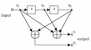
The plot above is a (2,1,2) convolution encoder. Usually we use (n,k,N) to specify a convolution encoder. So for the (2,1,2) encoder, the input information bits are stored in a N=2-stage register, when k=1 bit information is input, n=2 redundant codes are calculated as the output.
In this plot, the output c1,c2 are related to b1,b2,b3 by
![]()
![]()
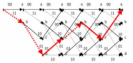
The plot below shows the state change and the output of a convolutional encoder. Here we assume that the initial state is b1b2b3=000. ‘a’、‘b’、‘c’、‘d’ here represent the value of b2b3 ‘00’、‘01’、‘10’ 、‘11’ respectively and the numbers on the line represent the output c1c2.
 plot
1
plot
1
The solid line in the plot shows the
state change when the input is ‘0’, while the dashed line shows the state change
when the input is ‘1’. Take the start point as an example, if the input is ‘0’,
then the new state becomes ‘00’, which is still state ‘a’ and the output is c1=0![]() 0
0![]() 0=0, c2=0
0=0, c2=0![]() 0=0;
if the input is ‘1’, then the new state will become ‘01’, which is state ‘b’ and
the output is c1=0
0=0;
if the input is ‘1’, then the new state will become ‘01’, which is state ‘b’ and
the output is c1=0![]() 0
0![]() 1=1, c2=0
1=1, c2=0![]() 1=1.
The red bold line shows the state change when the input sequence is ‘11010’,
also the output is showed on the line, which is ‘110101001011’.
1=1.
The red bold line shows the state change when the input sequence is ‘11010’,
also the output is showed on the line, which is ‘110101001011’.
Viterbi algorithm for decoding
How do we execute decoding?
Here we mainly discuss the Viterbi algorithm.
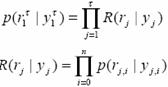
Assume that the original sequence is M{m1,m2,…,mM}, and the coded sequence is Y{y1,y2,…,yL}. So equation M/k=L/n hold, since for every k codes input, the convolutional encoder generate n codes, which are then transmitted. Assume that at the receiver, the detected signal sequence is R{r1,r2, …,rL}, so the conditional probability function is
![]()
Since at the receiver, we can only perceive R, we consider the sequence M’ that maximize the equation above as the output of the decoder. For computational convenience, we take log value:
![]()
And we define it as the path metric.
We use AWGN to describe the channel and assume that the transmitted sequence only take value ‘+1’ and ‘-1’, the energy is Es, the power spectral density of the noise is N0/2, so
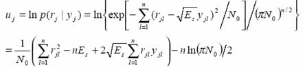
It is defined as the branch metric.
Since the energy for each code Es, the energy of the received data and the energy of the noise are the same, so we usually adopt
![]()
as the branch metric.
So the path metric, which is the sum of branch metric is:
![]()
The sequence M’ or Y’ that gives the maximum path metric is just the optimum solution for the detected output. Alternatively, if we have calculated the maximum path metric, we would get the decoded output, namely the transmitted sequence.
The specific procedure can be illustrated by the following plot.
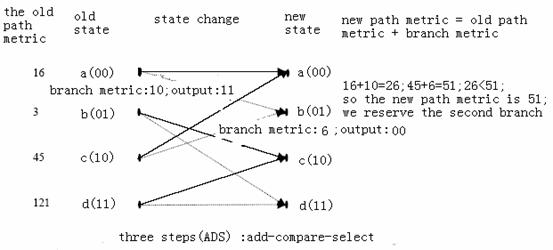
We can see that 2L(N+1) paths have to be calculated to get the decoded sequence, but we usually calculate only 5~7 times the constraint length and use the state 5~7 times constraint length before as the decoded output, since the correlation of the code 3~5 constraint length apart will be so small that it won’t have effect on the output detected code.
Turbo code
The advance of turbo code is a revolutionary innovation in coding technique.
The structure of the turbo encoder can be illustrated by the plot below.
MAP algorithm
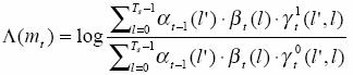
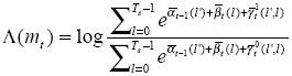
This algorithm uses a maximum a posterior probability to decide the output according to the received sequence. Still we use a log value.
![]()
Here 1≤t≤τ, τ is the length of the received sequence. Thus,
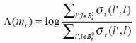
![]()
If Λ(mt)≥0, then Pr(mt=1|R)≥Pr(mt=0|R), so we consider mt=1; otherwise we think mt=0.
Assume that the original sequence is M{m1,m2,…,mL}, denoted as m1L, the encoded sequence is Y{y1,y2,…,yT}, denoted by y1T, and the received sequence R(r1T) is encoded sequence corrupted by a Gaussian white noise whose mean is 0 and variance is σ. Here we assume that k=1.
Assume that at time t, the state of the register is denoted by St, the received bit code is mt+1, the new state is St+1 and the output block is yt+1. We define
![]()
Ts is the number of states.
So the probability of output of the encoder is
![]()
We can perceive that Pt(l|l ’) is either 0.5 or 0. Since for each present state, there can only be to choices for the next state, determined by the input 1 or 0. And qt(yt| l ’, l ) is either 1 or 0, since the output is definitely determined when the old and new states are determined.
So the probability that the transmitted sequence is y1T and the received sequence is r1T is
Here n is the number of output when one bit information is input. And
![]()

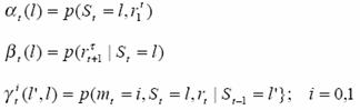
The a posterior probability is
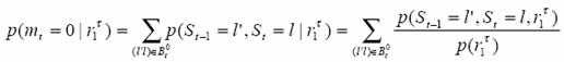
Here St-1 and St are all possible consecutive states that would correspond to an input ‘0’, the set of which is denoted as Bt0. Take plot 1 as an illustration, Bt0={(0,0),(2,0),(3,2),(1,2)}. Also

Here St-1 and St are all possible consecutive states that would correspond to an input ‘1’, the set of which is denoted as Bt1. In plot 1, Bt1={(0,1),(2,1),(3,3),(1,3)}.
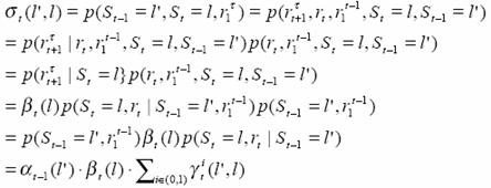
We define the a posterior probability (APP) as
![]()
So
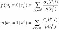
,and so
To calculate![]() , we
define
, we
define
,then
,and 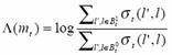
Calculate α
The boundary condition is
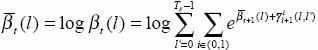
Calculate β
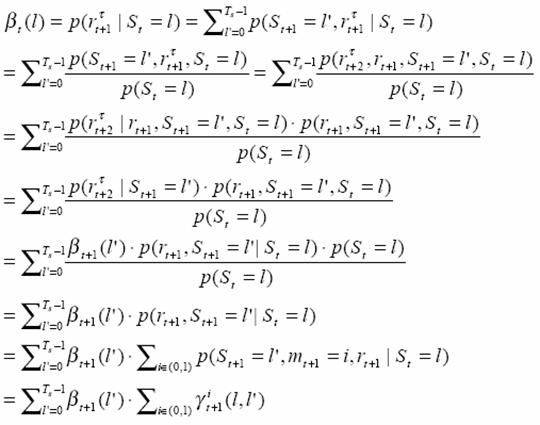
The boundary condition is
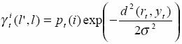
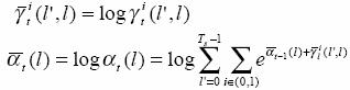
Calculate γ
Further we can get
Here ![]() is
the a priori probability,
is
the a priori probability, ![]() is
the output when state changes from
l
’ to
l
.
is
the output when state changes from
l
’ to
l
.
Note that R(rt|yt)
is multiplied by ![]() .
.
Summary to MAP algorithm
(1) Forward recursive
Initialize α0(l)
When ![]() , i=0,1,
calculate
, i=0,1,
calculate
Here ![]() is
the Euclidean distance between rt and yt.
is
the Euclidean distance between rt and yt.
Store ![]() .
.
For t=1,2,…,τ, l=0,1,2,…,Ts-1, calculate and store αt(l).
(2) Backward recursive
Initialize βt(l)
When t=τ-1,…,1,0, l=0,1,…,Ts-1
![]()
For t<τ
Max-Log-MAP
Usually, we use the log value for calculation simplicity
Thus
Since
![]()
![]()
Here the calculation for ![]() and
and ![]() are
the same as that for the path metric in Viterbi algorithm, and
are
the same as that for the path metric in Viterbi algorithm, and ![]() plays
the role of the branch metric.
plays
the role of the branch metric.
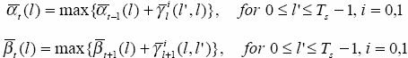
We call this the Max-Log-MAP.
Recursive decoding for turbo code using MAP algorithm
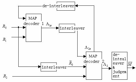
In the plot above, R0 and R1 enter the first MAP decoder, the output is first interleaved and then enters the second decoder as the a priori probability. R0 is then first interleaved and then enters the second MAP decoder together with R2. The output of the second decoder is first de-interleaved and then enters the first decoder as the a priori probability.
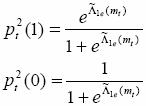
For the first MAP decoder,
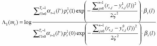
Here pt1(1) and pt1(0) are the a priori probability for input bit ‘1’ and ‘0’ for the first decoder.. Correspondingly, that of the second decoder are denoted as pt2(1) and pt2(0). We assume
![]()
when doing the first decoding for the first decoder. So
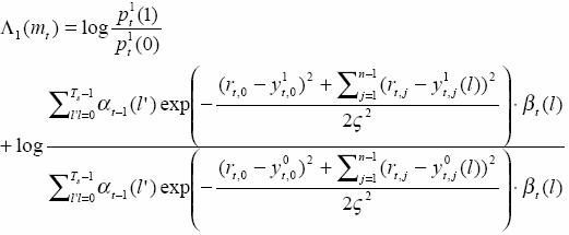
As ![]()
![]()
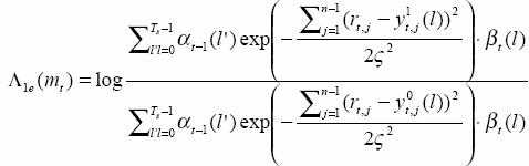
Here Λ1e(mt) is called additional information, since it does not include rt,0, it can be used as the a priori information for the second decoder. Namely
![]()
As ![]()
Similarly we can get the output of the second decoder

![]()
Λ2e(mt) is the additional information of the second decoder and can also be used as the priori information for the first decoder. So
![]()
Summary of recursive decoding for turbo code using MAP algorithm
(1)
initialize ![]()
(2) for r=1,2,,I, calculate
![]() and
and ![]()
![]()
![]()